Machine Learning Course Summary (Part 4)

Summary from the Stanford's Machine learning class by Andrew Ng

---

• Part 1
  • Supervised vs. Unsupervised learning, Linear Regression, Logistic Regression, Gradient Descent
• Part 2
  • Regularization, Neural Networks
• Part 3
  • Debugging and Diagnostic, Machine Learning System Design
• Part 4
  • Support Vector Machine, Kernels
• Part 5
  • K-means algorithm, Principal Component Analysis (PCA) algorithm
• Part 6
  • Anomaly detection, Multivariate Gaussian distribution
• Part 7
  • Recommender Systems, Collaborative filtering algorithm, Mean normalization
• Part 8
  • Stochastic gradient descent, Mini batch gradient descent, Map-reduce and data parallelism

---

Support Vector Machines

• Hypothesis and Decision Boundary 
  • Hypothesis 

• Decision Boundary

• Kernels
  • For Non Linear Decision Boundary we can use higher order polynomials but is there a different/better choice of the features ?
  • High order polynomials can be computationally heavy for image processing type problem.
  • Given X, compute new feature depending  on proximity to landmarks.

• When x = 3/5 the bump increases as its near to the landmark l(1), which is equal to [3,5], sigma square value makes the bump narrow or wide.

• Predict “1” when theta0 + theta1 f1 + theta2 f2 + theta3 f3  >= 0
• Let’s assume theta0 = -0.5, theta1 = 1, theta2 = 1, theta3 = 0
• For x(1),
  • f1 == 1 ( as its close to l(1))
  • f2 == 0 ( as its close to l(2))
  • f3 == 0 ( as its close to l(3))
• Hypothesis :
  • = theta0 + theta1 * 1 + theta2 * 0 + theta3 * 0
  • = -0.5 + 1
  • = 0.5  (which is > 0, so we predict 1 )

• How do we choose Landmarks ??
• What other similarity functions we can use other than ‘Gaussian Kernel” ??
  • * Make l same as X

• Kernels do not go well with logistic regression due to computational complexity
• SVM with Kernels are optimized for computation and runs much faster

Using SVM

Use software packages (liblinear, libsvm, …) to solve for parameters theta.

Need to Specify:

• Choice of parameter C
• Choice of Kernel (similarity function)
  1. No Kernel (“linear kernel”)
     • Predict “y=1” if theta transpose x > 0
     • No landmarks or features f(i) from x.
     • Choose this when n is large and m is small. (Number of features is large and training examples are less)
  2. Gaussian Kernel
     • Predict “y=1” if theta transpose f > 0
     • Use landmarks
     • Need to choose sigma square
     • Choose this when n is small and m is large. ( very large training set but small number of features)
     • Do perform feature scaling before using the Gaussian kernel
  3. Other choices
     • All similarity function need to satisfy a technical condition called “Mercers Theorem”
     • Polynomial kernel
     • More esoteric:
       1. string kernel
       2. chi-square kernel
       3. historgram intersection kernel

Many SVM packages already have built-in multi class classification functionality, if not use the one-vs-all method

• Logistic Regression vs. SVM

 

Machine Learning Course Summary (Part 2)

 

Summary from the Stanford's Machine learning class by Andrew Ng

---

• Part 1
  • Supervised vs. Unsupervised learning, Linear Regression, Logistic Regression, Gradient Descent
• Part 2
  • Regularization, Neural Networks
• Part 3
  • Debugging and Diagnostic, Machine Learning System Design
• Part 4
  • Support Vector Machine, Kernels
• Part 5
  • K-means algorithm, Principal Component Analysis (PCA) algorithm
• Part 6
  • Anomaly detection, Multivariate Gaussian distribution
• Part 7
  • Recommender Systems, Collaborative filtering algorithm, Mean normalization
• Part 8
  • Stochastic gradient descent, Mini batch gradient descent, Map-reduce and data parallelism

---

Regularization

• Problem of Overfitting

• Options to address overfitting:
  • Reduce number of features
    • Manually select which features to keep
    • Model selection algorithm (later in course)
  • Regularization
    • Keep all features but reduce magnitude/values of parameters theta.
    • works well when we have lots of features, each of which contributes a bit to predicting y.
• Too much regularization can “underfit” the training set and this can lead to worse performance even for examples not in the training set.

• Cost Function
  • if lamda is too large (e.g. 10¹⁰) than the algorithm results in “underfitting”(fails to fit even training set)

• Regularization with Liner Regression

• Normal Equation

• Regularization with Logistic Regression

Neural Networks

• Introduction

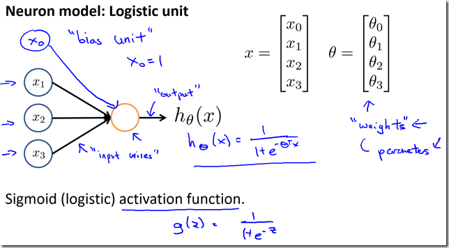
  • Algorithms that try to mimic the brain. Was very widely used in 80s and early 90s; popularity diminished in late 90s.

  • Send a signal to any brain sensor and it will learn to deal with it. E.g. Auditory cortex learns to see, Somatosensory cortex learn to see.
    Seeing with your tongue, human echolocation, third eye for frog.
    

• Model Representation

• Forward propagation

• Non-linear classification example: XOR/XNOR

• Non-linear classification example: AND

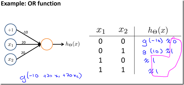
• Non-linear classification example: OR

• XNOR

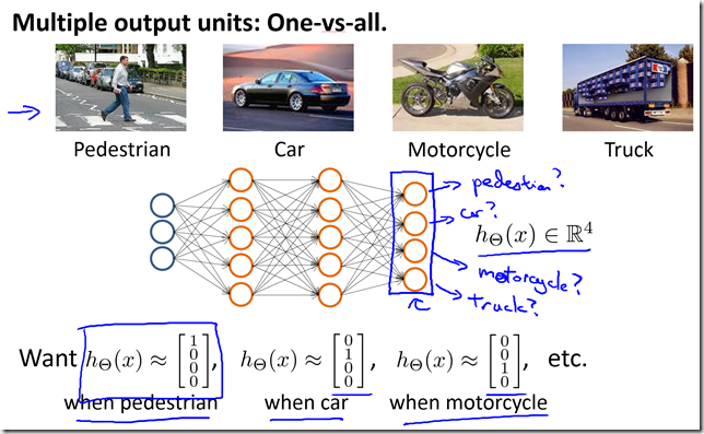
• Multi-class classification

• Cost Function

• Unlike logistic regression we DO NOT sum the value of “Bias Unit” in the regularization term for cost of neural networks.
• Just as logistic regression a large value of “lamda” will penalize large parameter values, thereby, reducing the changes of overfitting the training set.

• Backpropagation algorithm

• Unrolling parameters

• Gradient Checking
  • There may be bugs in forward/back propagation algorithms even if the cost function looks correct.
  • Gradient checking helps identify these bugs.

• Implementation Note:
  • Implement backprop to compute DVec (unrolled ).
  • Implement numerical gradient check to compute gradApprox.
  • Make sure they give similar values.
  • Turn off gradient checking. Using backprop code for learning
• Be sure to disable your gradient checking code before training your classifier. If you run numerical gradient computation on
  every iteration of gradient descent (or in the inner loop of costFunction(…))your code will be very slow.

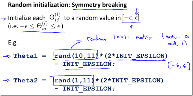
• Random initialization
  • Initializing theta to 0 works for logistic regression but it does not work for neural network.
  • If we initialize theta to 0 than for neural network, after each update, parameters corresponding to inputs going to each of two hidden units are identical.
  • This causes the “Problem of Symmetric Weight”
  • To solve this issue randomly initialize the theta values.

• Training a neural network

 

Machine Learning Course Summary (Part 3)

 

Summary from the Stanford's Machine learning class by Andrew Ng

---

• Part 1
  • Supervised vs. Unsupervised learning, Linear Regression, Logistic Regression, Gradient Descent
• Part 2
  • Regularization, Neural Networks
• Part 3
  • Debugging and Diagnostic, Machine Learning System Design
• Part 4
  • Support Vector Machine, Kernels
• Part 5
  • K-means algorithm, Principal Component Analysis (PCA) algorithm
• Part 6
  • Anomaly detection, Multivariate Gaussian distribution
• Part 7
  • Recommender Systems, Collaborative filtering algorithm, Mean normalization
• Part 8
  • Stochastic gradient descent, Mini batch gradient descent, Map-reduce and data parallelism

---

Debugging & Diagnostics

• Evaluating a Hypothesis
  • What if the hypothesis fails to generalize to new examples not in training set?
  • Divide the dataset into Train set, Cross Validation st and Test set

• Bias vs. Variance
  • Underfit, Just Right and Overfit graphs.

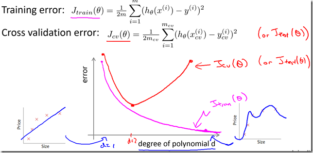
• Error graph comparing Cross validation error and Training error

• How to identify if it is a bias problem or a variance problem?

• Regularization and bias/variance
  • Large, Intermediate and Small lamda values.

• Choosing the regularization parameter “lamda”:

• Learning Curves

• Debugging 
  • Suppose you have implemented regularized linear regression to predict housing prices.
    However, when you test your hypothesis on a new set of houses, you find that it makes unacceptably large errors in its predictions. What should you try next?
    • Get more training examples ?  Fixes High Variance 
    • Try smaller sets of features ?  Fixes High Variance 
    • Try getting additional features ?  Fixes High Bias
    • Try adding polynomial features ?  Fixes High Bias
    • Try decreasing lamda ?  Fixes High Bias
    • Try increasing lamda ? Fixes High Variance 

• Neural networks and overfitting

Machine Learning System Design

• Prioritize What to work on
  • Spend your time to make it have low error
    • Collect lots of data (e.g. “honeypot” project)
    • Develop sophisticated features
    • Develop sophisticated algorithms
  • Error Analysis
    • Start with simple algorithm that you can implement quickly.
    • Plot learning curves to decide if more data, more feature etc. is likely to help.
    • Manually examine the examples in Cross Validation set, which our algorithm made errors on. See if we can find any systematic trend.
• Error Metrics for Skewed classes
  • Use this when you have more number of positive examples than negative examples.
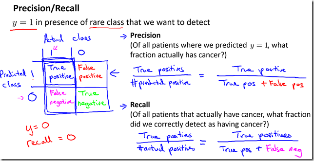
  • Precision / Recall
    • A classifier with high precision and high recall is good, even if we have very skewed classes.

• F₁ Score (F Score)

• Large Data Rationale
  • “It’s not who has the best algorithm that wins. It’s who has the most data.”